Temp

Monte Carlo Basics

Quite often we would like to know which of the proposed estimators is “better” and under what conditions. The exact answer (for any sample size) to these questions is known only for a quite limited class of estimators, distributions of error terms and regression functional forms. We can address these questions using various Central Limit Theorems. However, the applicability of our results relies on a “sufficiently large” number of observations for asymptotics to kick in. The question “When sufficiently large is large enough?” is a very interesting one, but it lies well beyond the scope of this discussion. In small samples asymptotics does not work. Unfortunately, this is exactly the area where all real-world applications belong to.

Monte Carlo method can somewhat address this issue. However, it has its own problems. Assume that we would like to know how the conditional quasi-maximum likelihood estimator (estimator A) performs compared to the unconditional quasi-maximum likelihood estimator (estimator B) for AR(1) process with AR coefficient [math]\alpha=.5[/math], sample size [math]T=50[/math] and t-distributed error terms with 10 degrees of freedom. On one hand, using MC method, we can reliably test the hypotheses that, for example, estimator A has smaller bias and/or smaller variance than estimator B. However, this answer, strictly speaking, can be applied only for the case of [math]\alpha=.5[/math], [math]T=50[/math], and t-disributed error term with 10 degrees of freedom. Once the sample size, autoregressive coefficient, degrees of freedom or distribution is changed, results might change significantly as well.

The idea behind the Monte Carlo Method is very simple. Assume for a moment that you can draw somehow observations from an (un)known distribution of interest. Then, by drawing sufficiently large number of observations from this distribution, you can approximate with an arbitrary level of precision:

1. finite population moments of any functions of random variables
2. CDF and/or pdf and thus quantiles of interest

As an example, for the case when the distribution is known and random number generator is readily available, we can compute

[math]E(|X|),E(|X|^3) \text{ for } X\sim N(0,1)[/math]

Formally, taking integrals we’ll get:

[math]\frac{1}{\sqrt{2\pi}}\int_{-\infty}^{\infty} |x|e^{-x^2/2}dx=\frac{2}{\sqrt{2\pi}}\int_{0}^{\infty} e^{-x^2/2}d(x^2/2)=\sqrt{\frac{2}{\pi}}\approx 0.7979[/math]

[math]\frac{1}{\sqrt{2\pi}}\int_{-\infty}^{\infty} |x|^3e^{-x^2/2}dx=\frac{2}{\sqrt{2\pi}}\int_{0}^{\infty} x^2e^{-x^2/2}d(x^2/2)=2\sqrt{\frac{2}{\pi}}\approx 1.5958[/math]

Alternatively, the Monte-Carlo algorithm to estimate [math]E(|X|)[/math] and [math]E(|X|^3)[/math] is:

1. Draw a large number (say, 10000000) of observations from a normal distribution [math]N(0,1)[/math] and compute [math]|x|[/math] and [math]|x|^3[/math] for each of them.
2. Take averages and report results

rng(1);x=randn(10000000,1);
absx=abs(x);
absx3=absx.^3;
disp([mean(absx) mean(absx3)])
     0.7982    1.5973

Which is quite close to the analytically evaluated ones. The more observations you take, the closer your results to the analytical ones will be.

However, in reality, the random number generator for the distribution of interest is not readily available. Quite often you have to construct it first.

OLS properties of AR(1) process estimator

Consider a very simple example: (un)biasedness of OLS estimator while applying it to AR(1) process

[math]y_t=\alpha y_{t-1}+e_t,\ e_t\sim N(0,\sigma^2)[/math]

Recall that the OLS estimator for regression

[math]y=X\beta+e, e\sim (0,\sigma^2_e I)[/math]

where [math]I[/math] is an identity matrix, is [math]\hat \beta=(X'X)^{-1}X'y=\beta+(X'X)^{-1}X'e[/math] Unbiasedness of OLS estimator, assuming [math](X'X)^{-1}[/math] exists, is satisfied as long as [math]E[(X'X)^{-1}X'e]=0[/math]. Sufficient condition for this to hold is [math]E(e|X)=0[/math]. While this is quite often the case for cross-sectional applications, this is definitely not the case for Time Series. The condition [math]E(e|X)=0[/math] has to be understood in the following way: any error term [math]e_s[/math] in this regression has to be independent from any [math]x_t[/math]. For AR processes, for obvious reasons, this is not the case. For example, [math]e_t[/math] is not independent from [math]x_{t+1}[/math] as [math]x_{t+1}[/math] is [math]y_t[/math]. [math]Cov(x_{t+1},e_t)=\sigma_e^2[/math]. Moreover, [math]Cov(x_{t+s},e_t)=\alpha^s\sigma_e^2[/math] and, thus the larger [math]|\alpha|[/math], the larger, presumably, has to be the bias. On the other hand, for consistency, it is sufficient that

[math]\label{consistency} (X'X/T)^{-1} \Rightarrow Q,\ X'e/T \Rightarrow 0[/math]

• where [math]Q[/math] is a full-rank finite matrix. Since these conditions are satisfied for covariance-stationary processes with gaussian increments, we expect that the bias will become smaller and smaller as the sample size increases.

Let’s sketch the algorithm:

1. Generate [math]y_t[/math] for [math]t=1,\ldots,T[/math], where [math]T=20[/math] and [math]\alpha=0[/math] using the following data generating process: [math]y_t=\alpha y_{t-1}+e_t[/math]
2. Estimate and save [math]\alpha[/math] using OLS (Please note, these steps correspond to the first step from the previous algorithm “draw a large number of observations from a distribution of interest)
3. Repeat pp 1-2 1000 times, compute [math]\bar{\hat{\alpha}}[/math] and bias
4. Repeat pp 1-3 for [math]\alpha=0.1, 0.2, ... , 0.9, 0.99[/math]
5. Repeat pp 1-4 for [math]T=50,100,200,1000[/math]
6. Plot results for different sample sizes

Before implementing the algorithm, we have to take care of one additional issue, i.e. sample simulation (p. 1). If we know [math]y_0[/math], we can generate [math]y_1[/math] drawing an observation from a normal distribution (using normal random number generator randn) and proceed to [math]y_T[/math].

[math]\begin{aligned} y_1&=\alpha y_{0}+e_1\\ y_2&=\alpha y_{1}+e_2\\ \ldots\\ y_T&=\alpha y_{T-1}+e_T\end{aligned}[/math]

• Unfortunately, [math]y_0[/math] is unknown. Please note: The whole discussion regarding [math]y_0[/math] below applies for processes with finite memory only. Compare with Random Walk.

One way to handle this problem is to pretend that [math]y_0[/math] is known, i.e. to assume that [math]y_0=E(y)=0[/math]. Then, [math]y_1=e_1[/math], [math]y_2=\alpha e_1+e_2[/math], etc. However, this approach has an additional issue. For AR(1) process [math]Var(y_t)=\frac{\sigma_e^2}{1-\alpha^2}[/math] for all [math]t[/math]. If we assume that [math]y_0=0[/math], however, [math]Var(y_1)=Var(e_1)=\sigma_e^2[/math], [math]Var(y_2)=\sigma_e^2(1+\alpha^2)[/math], and for arbitrary [math]t\gt 0[/math]: [math]Var(y_t)=\sigma_e^2\sum_{i=0}^{t-1}\alpha^{2(t-1)}=\sigma^2_e\frac{1-\alpha^{2t}}{1-\alpha^2}[/math]. For a reasonably large [math]t[/math]: [math]V(y_t)\approx\frac{\sigma^2_e}{1-\alpha^2}[/math]. Thus, if we decide to implement this algorithm, we have to start recording [math]y[/math] not from the first observation, but from some non-zero [math]T_0[/math] s.t. [math]\alpha^{2T_0}\approx 0[/math]. Obviously, [math]T_0[/math] depends on [math]\alpha[/math]. The larger [math]\alpha[/math], the larger [math]T_0[/math] should be. The thrown away part of the sample is sometimes called a “burn-in” period.

Alternatively, we can take into account the fact that [math]y_0[/math] is not known and generate [math]y_1[/math] directly with [math]E(y_1)=0[/math] and [math]Var(y_1)=\frac{\sigma^2_e}{1-\alpha^2}[/math], i.e. [math]y_1=e_1/\sqrt{1-\alpha^2}[/math]

For stationary processes the first approach does not require any analytical derivations, i.e. any knowledge of unconditional and various conditional population moments of the process. The second one runs faster. However, the second method has its own issues. It is easy to implement it for AR(1) process. For ARMA(p,q) the amount of effort increases significantly. For stochastic volatility models it might become unbearable.

I will focus on the first version. [math]T_0=200[/math] is sufficiently large for almost all values of [math]\alpha[/math] considered. The p.1 of the algorithm becomes:

1. Generate [math]y_t[/math] for [math]t=1,\ldots,T[/math], where [math]T=20[/math] and [math]\alpha=0[/math]
   1. Draw [math]T+T_0[/math] observations from [math]N(0,1)[/math] with [math]T_0=200[/math], save them in a vector [math]e[/math] and assume [math]z_0=0[/math]
   2. Construct [math]z_t[/math] for [math]t=1[/math]: [math]z_t=\alpha z_{t-1}+e_t[/math]
   3. Repeat 1.a) for [math]t=2,3,\ldots,T+T_0[/math]
   4. Save the last T observations as vector [math]y[/math]

To make the code easier to understand, we will write a set of functions for these steps. (Please see the section about functions). Also, we will use for .. end loop here. Please see the section about loops.

Lets implement the first step, i.e. generation of a sample of size [math]T[/math]. This function has to have three parameters: alpha, [math]T_0[/math], [math]T[/math]. We call it dgp, i.e. data generating process.

function y=dgp(alpha,T0,T)
Tt=T+T0;
e=randn(Tt,1); %1 a)
z=zeros(Tt,1);
z(1)=e(1); %since z_0=0
for t=2:Tt
    z(t)=alpha*z(t-1)+e(t);
end
y=z(end-T+1:end); %dropping first T0 observations
end

The next step is to construct an estimate for [math]\alpha[/math]:

function alpha=myar1(y)
X=y(1:end-1);%specifying X
y=y(2:end);%specifying y
alpha=inv(X'*X)*X'*y; %Estimating AR(1) parameter
end

The next step is to repeat these steps 1000 times, compute mean, bias and standard errors of [math]\hat\alpha[/math]. For the sake of generality, this function will depend on [math]T_0[/math], [math]T[/math], [math]\alpha[/math], [math]N[/math], where [math]N[/math] - number of replication, in our case 1000.

function [meanalpha biasalpha stdalpha]=MC(alpha,T0,T,N)
 for i=N:-1:1
 %This way we don't need to initialize alphahat vector prior to the cycle
    y=dgp(alpha,T0,T);
    alphahat(i,1)=myar1(y);
 end
meanalpha=mean(alphahat);
biasalpha=mean(alphahat-alpha);
stdalpha=std(alphahat);
end

The next step is to repeat our simulations for different sample sizes and different alphas. The easiest way is to create two vectors of values, one for different sample sizes, one for different alphas, and loop over all possible combinations of them:

alphavec=[0:.1:.9 .99];
Tvec=[20 50 100 200 1000];
T0=200; %burn-in period
N=1000; %number of iterations
rng(1); %for results replicability
for Tind=1:length(Tvec)
  T=Tvec(Tind); %picking the right T
  for alphaind=1:length(alphavec)
      alpha=alphavec(alphaind); %picking the right alpha
      [meanalpha(alphaind,Tind) biasalpha(alphaind,Tind) stdalpha(alphaind,Tind)]=MC(alpha,T0,T,N);
  end
end

And the last, but not the least, step is to plot our results:

plot(alphavec,biasalpha)
title('Bias as a function of sample size and $\alpha$','interpreter','latex')
xlabel('$\alpha$','interpreter','latex')
ylabel('Bias of $\hat\alpha$','interpreter','latex')
legend({'T=20','T=50','T=100', 'T=200', 'T=1000'})
figure
plot(alphavec,stdalpha)
title('Standard error of $\hat\alpha$ as a function of sample size and $\alpha$','interpreter','latex')
xlabel('$\alpha$','interpreter','latex')
ylabel('Std of $\hat\alpha$','interpreter','latex')
legend({'T=20','T=50','T=100', 'T=200', 'T=1000'})

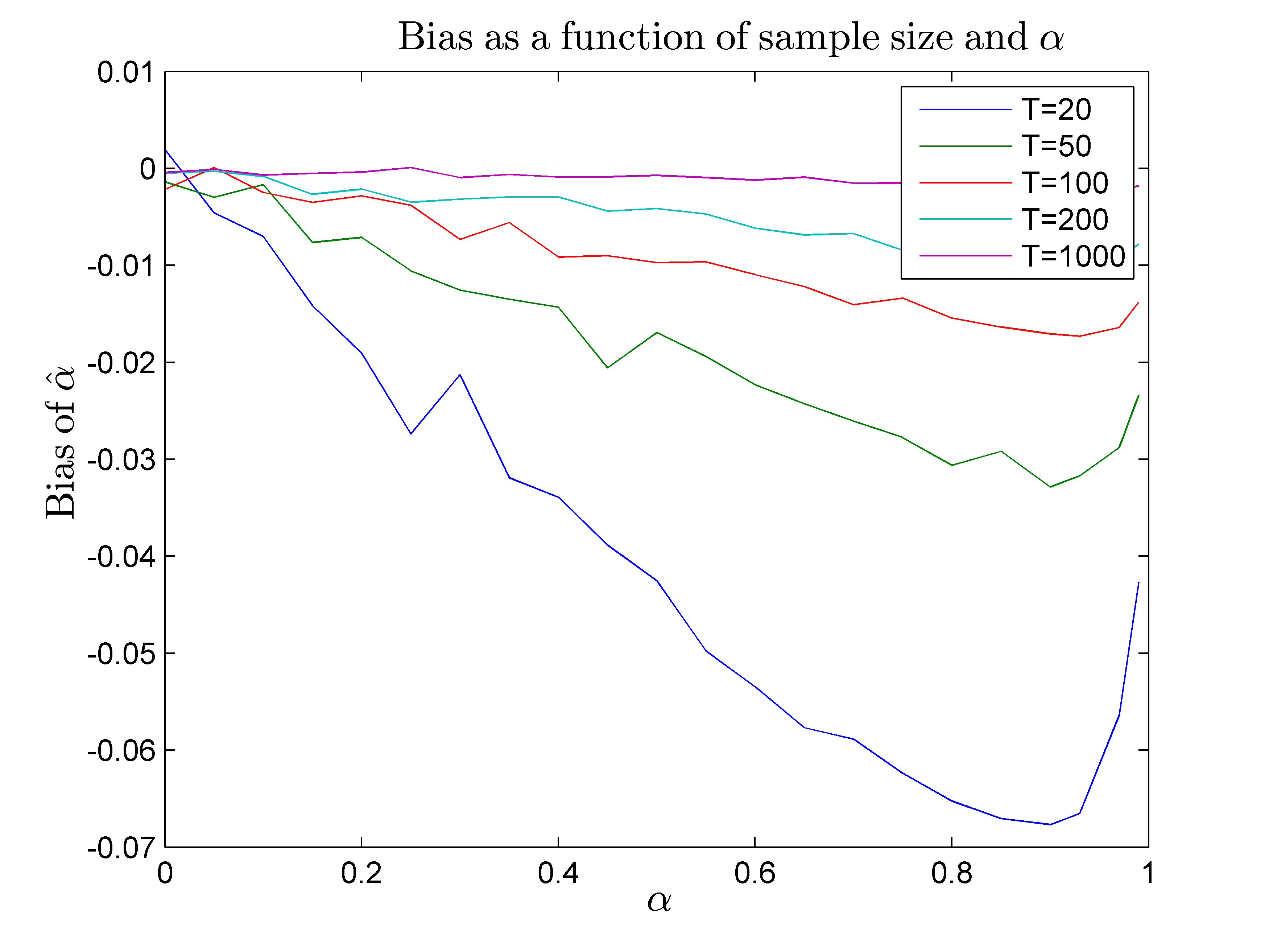
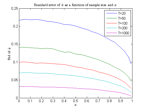
The next two figures are generated using the code above. To create a smoother picture, we ran simulations for [math]N=10000[/math], [math]\alpha=0,0.05,0.1,0,15,\ldots,0.95,0.99[/math]

Some of the findings coincide with our predictions, some of them do not. In particular,

1. Bias of [math]\alpha=0[/math] is very close to 0
2. Bias of [math]\alpha[/math] increases (in absolute value) up to some point
3. Standard errors decrease (Figure 2) as sample size increases.

One outcome that contradicts our “intuition” is the fact that bias in absolute value decreases after some point. This point depends on the sample size. The intuition for this behavior lies in the notion of non-stationarity. As [math]\alpha[/math] further and further increases, stationary series start to behave more and more like non-stationary ones. For non-stationary time series [math]X'X/T^2=\sum y_t^2 /T^2 \Rightarrow C(B(t))[/math], while [math]X'e/T = \sum y_{t-1}e_t/T \Rightarrow C'(B(t))[/math], where [math]C(B(t)),C'(B(t))[/math] – finite functionals of Brownian motions. Thus, for [math]|\rho|\rightarrow 1[/math], [math](X'X)^{-1}[/math] will dominate [math]X'y[/math] and the bias will decrease. Moreover, for [math]\rho=1[/math], [math]\hat\alpha[/math] is a consistent estimator of [math]\alpha[/math] even in the case of [math]Cov(x_t,e_t)\ne 0[/math].

On a notion of conditionality

Repeat simulation using a slightly modified version of the main code, i.e. 

alphavec=[0:.1:.9 .99];
Tvec=[20 50 100 200 1000];
T0=200; %burn-in period
N=1000; %number of iterations
%rng(1); %for results replicability
for Tind=1:length(Tvec)
  T=Tvec(Tind); %picking the right T
  for alphaind=1:length(alphavec)
      rng(1); %this is the new line 
      alpha=alphavec(alphaind); %picking the right alpha
      [meanalpha(alphaind,Tind) biasalpha(alphaind,Tind) stdalpha(alphaind,Tind)]=MC(alpha,T0,T,N);
  end
end

Compare the smoothness of the graphs. Explain the differences.