R TS VAR
Contents
Introduction
Here we will demonstrate how to use R to model multivariate time series in a Vector Autoregressive Model (VAR).
There are a variety of ways to deal with time-series datasets in R. As discussed in another section of the ECLR webpage we could use the standard ts format.
In addition to treating the data as time-series objects we will need a package that does the hard lifting in terms of estimating the VAR, testing the model specification, producing forecasts or creating impulse response functions. Should these terms not make any sense to you then you should stop reading here and proceed by learning about VARs. Here we only show how to implement them in R. The package we use for this is the vars package (written by Bernard Pfaff) and hence, before you do anything else you shouldcheck whether you already have this package or whether you need to install it.
install.packages("vars")
We then proceed by loading a few packages we need:
setwd("T:/ECLR/R/VAR") # replace with your working directory
library(xts)
library(vars)
Import Data
We use 10year maturity yields for the US, UK, German and French government bonds. The data come from the FRED database: UK, US, Germany and France.
We will use thge montly data from January 1975 to March 2015. These data are saved in a csv file with the four columns of data (LongRates.csv).
rates <- read.csv("LongRates.csv")
Let's have a look at what these data look like:
head(rates)
##         DATE   US Germany    UK France
## 1 01/01/1975 7.50     9.4 15.07  10.90
## 2 01/02/1975 7.39     8.9 13.33  10.69
## 3 01/03/1975 7.73     8.9 12.24  10.34
## 4 01/04/1975 8.23     8.8 12.42  10.36
## 5 01/05/1975 8.06     8.6 13.11  10.31
## 6 01/06/1975 7.86     8.4 12.99  10.21
Transforming into (m)ts format
Before we get cracking we want to ensure that the data are recognised as time-series data. Here we use the ts class which has also been used on the page for univariate modelling.
We first pick each individual country's rate
ger <- ts(rates$Germany, start=c(1975, 1), end=c(2015, 3), frequency=12)
fra <- ts(rates$France, start=c(1975, 1), end=c(2015, 3), frequency=12)
uk <- ts(rates$UK, start=c(1975, 1), end=c(2015, 3), frequency=12)
us <- ts(rates$US, start=c(1975, 1), end=c(2015, 3), frequency=12)
rates.ts = cbind(us,ger,uk,fra)
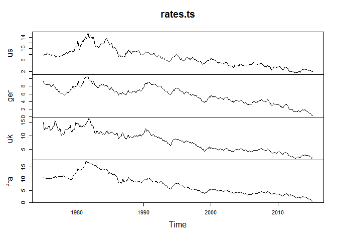
And let's look at a plot of these series:
plot(rates.ts)
In addition to the levels we shall also prepare an object with the differenced series.
drates.ts <- diff(rates.ts)
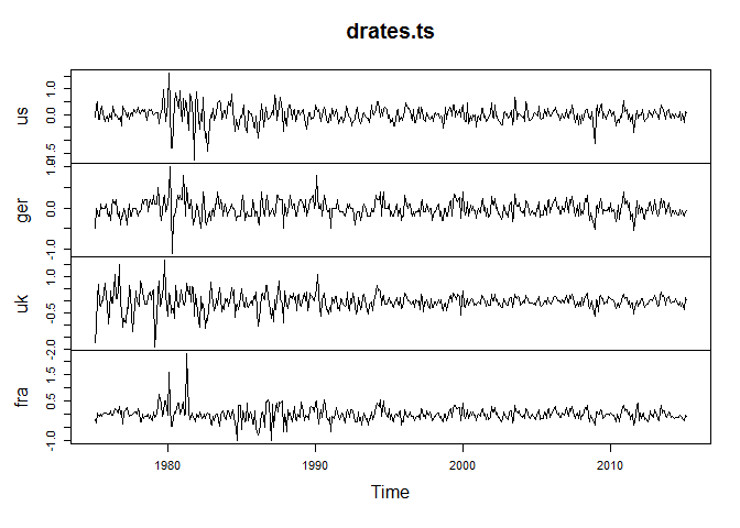
And let's look at a plot of these series:
plot(drates.ts)
Some preliminary data analysis
Before you embark on a VAR analysis you may want to establish that the order of integration of your time series. You could, e.g., perform a unit root test for the German long rates. This can be done with the ur.df function which performs an Augmented Dickey-Fuller (ADF) test.
summary(ur.df(rates.ts[, "ger"], type = "trend", lags = 2))
##
## ###############################################
## # Augmented Dickey-Fuller Test Unit Root Test #
## ###############################################
##
## Test regression trend
##
##
## Call:
## lm(formula = z.diff ~ z.lag.1 + 1 + tt + z.diff.lag)
##
## Residuals:
##      Min       1Q   Median       3Q      Max
## -0.96955 -0.12064 -0.00951  0.11437  0.86609
##
## Coefficients:
##               Estimate Std. Error t value Pr(>|t|)
## (Intercept)  0.1609140  0.0758616   2.121   0.0344 *
## z.lag.1     -0.0177337  0.0079895  -2.220   0.0269 *
## tt          -0.0002992  0.0001306  -2.291   0.0224 *
## z.diff.lag1  0.3776531  0.0453528   8.327 8.92e-16 ***
## z.diff.lag2 -0.1055146  0.0454611  -2.321   0.0207 *
## ---
## Signif. codes:  0 '***' 0.001 '**' 0.01 '*' 0.05 '.' 0.1 ' ' 1
##
## Residual standard error: 0.1869 on 475 degrees of freedom
## Multiple R-squared:  0.1337, Adjusted R-squared:  0.1264
## F-statistic: 18.33 on 4 and 475 DF,  p-value: 5.115e-14
##
##
## Value of test-statistic is: -2.2196 2.6479 2.7133
##
## Critical values for test statistics:
##       1pct  5pct 10pct
## tau3 -3.98 -3.42 -3.13
## phi2  6.15  4.71  4.05
## phi3  8.34  6.30  5.36
If you know your unit root tests you can see that in this case we cannot reject the Null hypothesis of non-stationarity of this time series. You will find similar results for the other series.
Opinions on whether you should apply the VAR model to stationary or non-stationary data diverge somewhat with proponents on both sides. This is not the place for this debate. Here we decide to estimate a VAR model on stationary series and hence we will from now on use the differenced dataset drates.ts. (Of course you should confirm that the first differences are indeed stationary!)
Estimating a VAR
Now we demonstrate how to estimate the VAR in R.
Lag selection
One of the first things you ought to check when estimating a VAR is how many lags you should use. We usually use the lag length that minimises some selection of information criterium. This is very easily done with the VARselect function. The options lag.max = 8 and type = "const" indicate that we are looking for up to 8 lags and that we chose to include a constant as a deterministic variable into the VAR model. As usual use ?VARselect to get details on the optional inputs.
VARselect(drates.ts, lag.max = 8, type = "const")
## $selection
## AIC(n)  HQ(n)  SC(n) FPE(n)
##      7      3      1      7
##
## $criteria
##                    1             2             3             4
## AIC(n) -1.165290e+01 -1.172625e+01 -1.178755e+01 -1.177210e+01
## HQ(n)  -1.158385e+01 -1.160196e+01 -1.160802e+01 -1.153732e+01
## SC(n)  -1.147732e+01 -1.141021e+01 -1.133105e+01 -1.117513e+01
## FPE(n)  8.693850e-06  8.079051e-06  7.598975e-06  7.717867e-06
##                    5             6             7             8
## AIC(n) -1.180622e+01 -1.179959e+01 -1.182123e+01 -1.181627e+01
## HQ(n)  -1.151620e+01 -1.145433e+01 -1.142073e+01 -1.136053e+01
## SC(n)  -1.106879e+01 -1.092170e+01 -1.080288e+01 -1.065746e+01
## FPE(n)  7.459759e-06  7.510543e-06  7.351413e-06  7.390077e-06
We can see that the different criteria select different lag lengths, e.g. the Hannan-Quinn Criterion (HQ) selects a lag length of 3, the Scwartz criterion (SC) selects a lag length of 1. Without any further consideration we shall from now on use lag length p = 1, mainly to reduce the size of the output in this illustration.
Series ordering
For those of you in the know, you know that when using VARs (in particular when producing impulse response functions (see below) the order of the time-series plays an important role. Looking at the object drates.ts you will recognise that the order is us, ger, uk, fra.
We will later see how to re-order these.
Model Estimation
The function that does the heavy lifting is the VAR function. Let's estimate a VAR of order 3 (p = 3) for the rate differences, including a constant (type = "const"), but no trend into the VAR.
mod1 <- VAR(drates.ts, p = 1, type = "const")
This saves the estimated model in the object mod1, and we can show some basic output using the summary(mod1) command. The output below shows all estimated parameters in all 4 equations as well as covariance and correlation matrices of the estimated residuals.
summary(mod1)
##
## VAR Estimation Results:
## =========================
## Endogenous variables: us, ger, uk, fra
## Deterministic variables: const
## Sample size: 481
## Log Likelihood: 91.372
## Roots of the characteristic polynomial:
## 0.3174 0.3174 0.2176 0.1231
## Call:
## VAR(y = drates.ts, p = 1, type = "const")
##
##
## Estimation results for equation us:
## ===================================
## us = us.l1 + ger.l1 + uk.l1 + fra.l1 + const
##
##        Estimate Std. Error t value Pr(>|t|)
## us.l1   0.36999    0.05337   6.933 1.35e-11 ***
## ger.l1 -0.12640    0.09478  -1.334    0.183
## uk.l1  -0.03706    0.04430  -0.837    0.403
## fra.l1 -0.01611    0.06559  -0.246    0.806
## const  -0.01064    0.01383  -0.770    0.442
## ---
## Signif. codes:  0 '***' 0.001 '**' 0.01 '*' 0.05 '.' 0.1 ' ' 1
##
##
## Residual standard error: 0.3015 on 476 degrees of freedom
## Multiple R-Squared: 0.1012,  Adjusted R-squared: 0.09366
## F-statistic:  13.4 on 4 and 476 DF,  p-value: 2.343e-10
##
##
## Estimation results for equation ger:
## ====================================
## ger = us.l1 + ger.l1 + uk.l1 + fra.l1 + const
##
##         Estimate Std. Error t value Pr(>|t|)
## us.l1   0.180016   0.032313   5.571 4.24e-08 ***
## ger.l1  0.139877   0.057391   2.437   0.0152 *
## uk.l1   0.027049   0.026823   1.008   0.3138
## fra.l1  0.012978   0.039717   0.327   0.7440
## const  -0.012285   0.008372  -1.467   0.1429
## ---
## Signif. codes:  0 '***' 0.001 '**' 0.01 '*' 0.05 '.' 0.1 ' ' 1
##
##
## Residual standard error: 0.1825 on 476 degrees of freedom
## Multiple R-Squared: 0.1724,  Adjusted R-squared: 0.1655
## F-statistic:  24.8 on 4 and 476 DF,  p-value: < 2.2e-16
##
##
## Estimation results for equation uk:
## ===================================
## uk = us.l1 + ger.l1 + uk.l1 + fra.l1 + const
##
##        Estimate Std. Error t value Pr(>|t|)
## us.l1   0.09500    0.05858   1.622    0.105
## ger.l1  0.08155    0.10403   0.784    0.433
## uk.l1   0.27351    0.04862   5.625 3.17e-08 ***
## fra.l1 -0.05724    0.07200  -0.795    0.427
## const  -0.01499    0.01518  -0.988    0.324
## ---
## Signif. codes:  0 '***' 0.001 '**' 0.01 '*' 0.05 '.' 0.1 ' ' 1
##
##
## Residual standard error: 0.3309 on 476 degrees of freedom
## Multiple R-Squared: 0.1093,  Adjusted R-squared: 0.1018
## F-statistic:  14.6 on 4 and 476 DF,  p-value: 2.968e-11
##
##
## Estimation results for equation fra:
## ====================================
## fra = us.l1 + ger.l1 + uk.l1 + fra.l1 + const
##
##         Estimate Std. Error t value Pr(>|t|)
## us.l1   0.176852   0.044794   3.948 9.07e-05 ***
## ger.l1 -0.006145   0.079558  -0.077    0.938
## uk.l1   0.010742   0.037184   0.289    0.773
## fra.l1  0.134449   0.055057   2.442    0.015 *
## const  -0.016074   0.011606  -1.385    0.167
## ---
## Signif. codes:  0 '***' 0.001 '**' 0.01 '*' 0.05 '.' 0.1 ' ' 1
##
##
## Residual standard error: 0.253 on 476 degrees of freedom
## Multiple R-Squared: 0.08913, Adjusted R-squared: 0.08147
## F-statistic: 11.64 on 4 and 476 DF,  p-value: 4.985e-09
##
##
##
## Covariance matrix of residuals:
##          us     ger      uk     fra
## us  0.09088 0.02886 0.03777 0.02879
## ger 0.02886 0.03332 0.02343 0.02470
## uk  0.03777 0.02343 0.10948 0.03152
## fra 0.02879 0.02470 0.03152 0.06402
##
## Correlation matrix of residuals:
##         us    ger     uk    fra
## us  1.0000 0.5244 0.3787 0.3775
## ger 0.5244 1.0000 0.3880 0.5347
## uk  0.3787 0.3880 1.0000 0.3765
## fra 0.3775 0.5347 0.3765 1.0000
Specification testing
We will often be concerned whether the chosen lag length was sufficiently large to capture all the systematic temporal correlation in the time-series. In case it is not we should expect to find a certain degree of autocorrelation in the estimated residuals.
So, we need to find to know how to test for resdual autocorrelation. Please use the help function to read about the parameter choices. lags.pt = 12 selects the maximum order of autocorrelation that is being tested for.
ser12 <- serial.test(mod1, lags.pt = 12, type = "PT.asymptotic")
print(ser12)
##
##  Portmanteau Test (asymptotic)
##
## data:  Residuals of VAR object mod1
## Chi-squared = 380.75, df = 176, p-value < 2.2e-16
## $serial
##
##  Portmanteau Test (asymptotic)
##
## data:  Residuals of VAR object mod1
## Chi-squared = 380.75, df = 176, p-value < 2.2e-16
The p-value is very small indicating that the null hypothesis of no autocorrelation is rejected. This is a signal that we really ought to increase tha lag length. Incidentally, it turns out that only once you choose VAR orders of 7 or higher residual autocorrelation is by and large eliminated. Despite this we shall continue working with the very basic VAR(1) model.
Impulse Response Functions (IRF) and re-ordering
One way in which VAR models are used is by interpreting the impulse response functions. To do this we use the irf function. When looking at the output of the estimated model mod1 we could see that the estimated residuals are quite strongly correlated with each other. This means that it is very important to generate orthogonal impulse response functions. The standard way to do that is by employing a Cholesky decomposition (option ortho = TRUE in the irf function).
irf1 <- irf(mod1, impulse = "ger", response = c("us", "ger", "uk", "fra"), ortho = TRUE, n.ahead = 6)
In this function call the option impulse = "ger" specifies that we are looking at German shocks and response = c("us", "ger", "uk", "fra") indicates for which series we want to see the IRF.
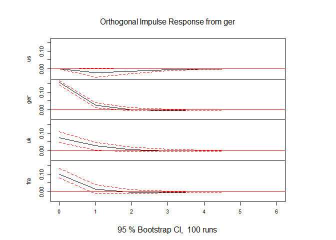
This saves the impulse response function in irf1. You can either print the values by print(irf1), or, more pleasingly plot them.
plot(irf1)
Here we can see that the strongest impact of a German shock is to the German long rate. UK and France rates also react but not as strongly. The US rate doesn't reacht immeadiately and barely after that. The fact that the US rate doesn't react to a German shock in the period of the shock (period 0) is by design. Recall that the ordering of the series is (US, GER, UK, FRA) implying that in the shock period a German shock cannot impact on the US rate.
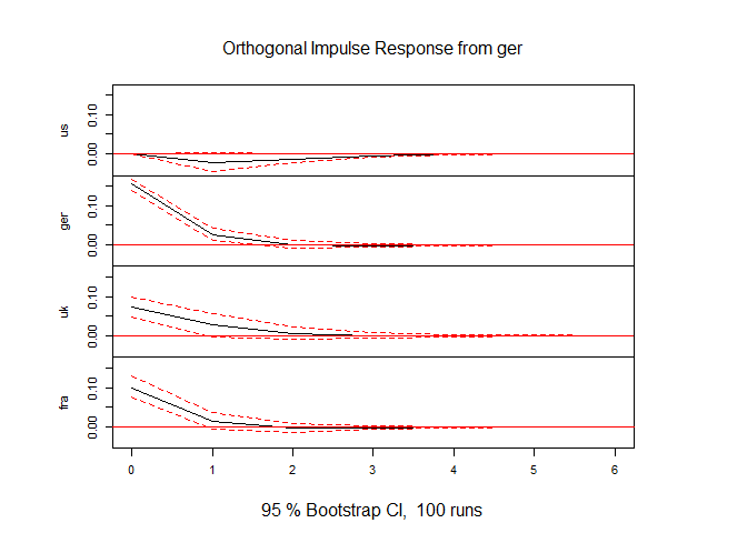
Of course we may want to change the ordering and re-evaluate the IRF. In the next block of code we first re-order (change the position of US and GER), then re-estimate and present the IRF for the new ordering.
drates.ts <- drates.ts[,c("ger","us","uk","fra")]
mod1r <- VAR(drates.ts, p = 1, type = "const")
irf1r <- irf(mod1, impulse = "ger", response = c("us", "ger", "uk", "fra"), ortho = TRUE, n.ahead = 6)
plot(irf1r)
As it turns out, even though now the US could react instantaneously to a GER shock, it doesn't. This indicates that the ordering of th US at the top of the heap is justified in this instance.
Some more resources
A few good resources are here:
- A detailed document on the
varspackage by its creator Bernard Pfaff can be found here.


